Course FAQ

Questions about tools and techniques that come up throughout the course, not only in the final project: sourcing data that is hard to find, querying OpenStreetMap, diagramming a workflow, and making an analysis more robust.

For questions specific to the final project — groups, the proposal, scoping, and past submissions — see the Final Project FAQ.

I’d like to create a conceptual diagram to describe my research process. What tools or models are available for me to do this?
I need point of interest data or data about features, but I can’t seem to find it from the local government, state/federal agency OpenData Hub… where else might I find it?
I checked everywhere and I can’t seem to find the map features (e.g., roads, business locations, bus stops, sidewalks, paths, parks, landmarks) I’m looking for. Where can I find them?
How do I make my analysis more rigorous than just describing the data?

Q: I’d like to create a conceptual diagram to describe my research process. What tools or models are available for me to do this?

A: You can use tools like PowerPoint or draw.io or Miro board to create conceptual diagrams for your analysis process. You can find some helpful examples of conceptual diagrams as well as detailed analysis diagrams in the Ranjit Kumar reading cited in the previous question.

Q: I need point of interest data or data about features, but I can’t seem to find it from the local government, state/federal agency OpenData Hub… where else might I find it?

A: It is not uncommon to hit roadblocks in accessing certain types of data at the federal level. Some of the most common data that this roadblock is encountered for is finding particular types of features like grocery stores, trails, or local landmarks. The following are a few alternative places you might look for this data:

Official governing documents (not georeferenced) — Often presented in PDF format, this data is not geographically referenced, but can be converted into tabular format (CSV), and with some follow-up validation after it is datafied it can be integrated into your analysis. Many governing authorities publish this information on their websites, but not explicitly on their OpenData portals.
ArcGIS Online Living Atlas — consolidates a wide array of authoritative data sources originated by both government agencies and reputable nongovernmental organizations. You can browse contents of the Living Atlas on ArcGIS Online and add data from the Living Atlas into ArcGIS Pro.
OpenStreetMap via Overpass Turbo — OpenStreetMap (OSM) is a decades-long crowdsourced project dedicated to creation and distribution of free geographic data worldwide. Learning to query OSM is a great skill to develop as a planner due to the wealth of geographically referenced data available through the project. There are numerous Python libraries that allow users to query the platform, however there exists a handy tool, Overpass Turbo, that allows users with minimal or no coding knowledge to query the tool. Navigate to the tool and click on the “Help” button in the top left corner of the interface or ask Li during Office Hours or a final project working session during class for more information.

Note: If you have some coding background, it is strongly recommended that you try out the newer Overture Maps utility which combines data from OpenStreetMap with other reputable sources and presents a more comprehensive cache of data (POI, roadways, etc.)

Q: I checked everywhere and I can’t seem to find the map features (e.g., roads, business locations, bus stops, sidewalks, paths, parks, landmarks) I’m looking for. Where can I find them?

A: You can export data from OpenStreetMap:

Check to see that the map features you are looking for are available via OSM using this Wiki with a detailed catalog of OSM map features: wiki.openstreetmap.org/wiki/Map_features
Once you have identified the features you would like to extract, navigate to Overpass Turbo, a web-based tool for filtering OSM data: overpass-turbo.eu

Note: This tool allows you to run API queries via Overpass and view/download outputted OSM data interactively on a map.
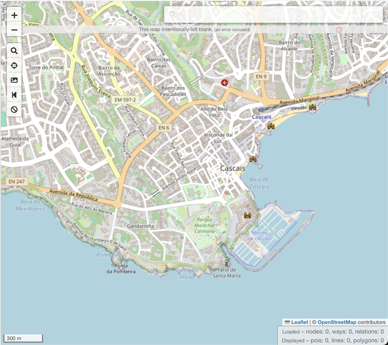
In the map to the right of your screen, navigate to the exact view extent for which you would like to extract map data. For example, if I wanted to extract all of the locations of grocery stores in Cascais, Portugal I would navigate to the extent of the jurisdictional bounds of Cascais…
You will need to construct a query to extract the map features you identified in Step 1. If I wanted to extract all of the locations of active supermarkets in Cascais, I would use the following syntax: shop=supermarket

To construct a query, you will need to take a few minutes to review how to construct basic queries using the wizard here: wiki.openstreetmap.org/wiki/Overpass_turbo/Wizard

If you are interested in constructing more advanced queries, you can review a few examples here: wiki.openstreetmap.org/wiki/Overpass_turbo/Examples

Note: If you are uncertain about the statement you’ve written you can always ask Li for help with the syntax during class!
Once you have constructed your query, click on the “Wizard” button on the toolbar in Overpass Turbo at the top of your browser viewport:

Note the additional examples provided in the Wizard pop-up. Does your query resemble them?
Enter your query text in the Search field beneath the examples then click “Build and Run Query.”

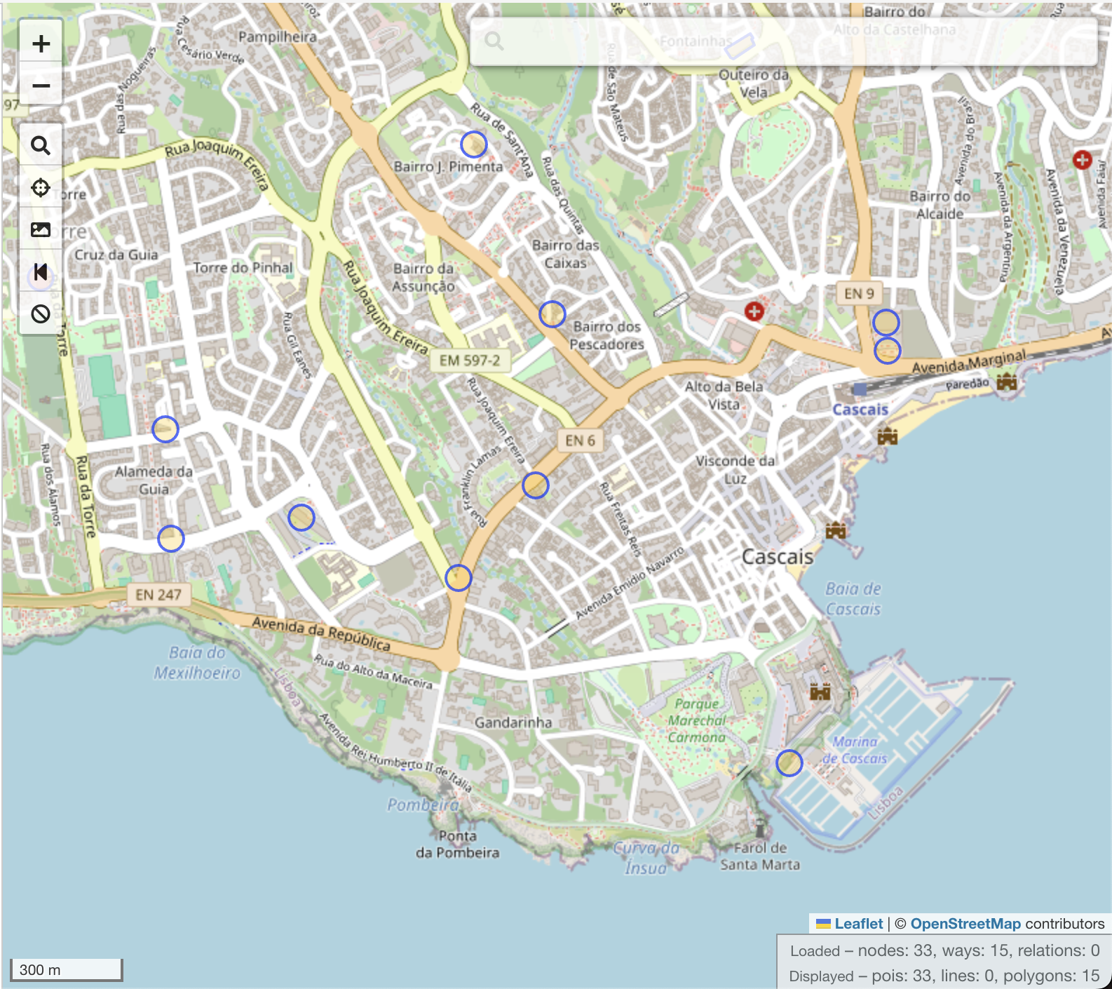
The results of your query will populate for your chosen map extent. Here are the results of my query for supermarkets in Cascais symbolized by circles with blue outlines:
The final step of this process is downloading the results of your query. Just click on the “Export” button in the toolbar at the top of your browser’s viewport in Overpass Turbo:
Select “GeoJSON” under the “Data” header:

Q: How do I make my analysis more rigorous than just describing the data?

A: If you have been told your analysis needs to be more robust, it usually means the work stops at description — reporting what the data contains — without testing whether the patterns you are pointing at are real.

Three levels of measure are listed below, each stronger than the last. Work down the list as far as your question needs. All of them run in Python, and you should report the statistic and what it tells you about your research question, not just the number.

Describe your inputs so the reader knows what the data looks like before any analysis.
Test relationships between variables to check whether an apparent association holds up.
Test spatial relationships to check whether the clustering you see on a map is more than chance.

1. Basic descriptives for input data

Python packages/functions (must have pandas or scipy imported into environment):

pandas.DataFrame.describe() — count, mean, std, min/max, quartiles in one call
numpy statistics routines — mean, median, std, percentile, etc.
scipy.stats.describe() — adds skewness and kurtosis to the basics

2. Correlation between two variables (not spatial)

Python packages/functions (must have scipy/pandas imported into environment):

scipy.stats.pearsonr() — linear (Pearson) correlation with p-value
scipy.stats.spearmanr() — rank-based (Spearman) correlation, useful for non-linear monotonic relationships
pandas.DataFrame.corr() — quick correlation matrix across many fields at once

3. Spatial autocorrelation (Moran’s I, Getis-Ord)

Sometimes it is necessary to look specifically at the spatial relationships between your variables — not just their location-agnostic characteristics/distributions. To do this you can use a few measures for spatial autocorrelation which test whether nearby features (geometry on the map) are more similar to each other than one might expect based on random chance.

Python packages/functions (must have libpysal and esda imported into environment; check whether install is necessary in Colab):

esda.Moran — looks at overall spatial autocorrelation (high next to high values, low next to low, etc.). A high value (close to 1) means high clustering, a low value (close to 0) means random, and negative values closer to -1 indicate strong dispersion.
esda.G — Global Getis-Ord statistics look for outliers in the data (consistently high or consistently low values for the entire dataset)
libpysal.weights — build the spatial weights matrix (contiguity, distance-band, k-nearest-neighbor) that all of the above require

When using this you will need to select the appropriate weights builder for the analysis if you are not just looking at the spatial relationship (weighting based on an input variable):

Queen — for polygons (swap in the template script for points below)
KNN (K nearest neighbors) — for points

Template script (for points):

import libpysal
import esda

shp = "stores.shp"  # path to your point shapefile
field = "SALES"  # the attribute field to test

w = libpysal.weights.KNN.from_shapefile(shp, k=6)
w.transform = "r"

y = libpysal.io.open(shp.replace(".shp", ".dbf")).by_col(field)

moran = esda.Moran(y, w)
print("Moran's I:", moran.I)
print("p-value:", moran.p_sim)

Acknowledgement: Thanks to Lian Plass for their help compiling these questions.